PIV computation

In this tutorial, we will see how to compute PIV (Particle Image Velocimetry) fields and how to load the results. In Fluidimage, we have the concept of “works” and “topologies” of works. Computing the PIV from 2 images is a “work” (defined in fluidimage.piv.Work). The PIV topology (fluidimage.piv.Topology) uses in the background the PIV work and also takes care of reading the images, creating the couples of images and saving the results.

A Fluidimage topology can be executed with different executors, which usually runs the different tasks in parallel.

Finding good parameters

In order to look for good parameters, we usually compute only PIV fields just with the PIV work fluidimage.piv.Work (i.e. without topology).

from fluidimage import get_path_image_samples
from fluidimage.piv import Work

We use the class function create_default_params to create an object containing the parameters.

params = Work.create_default_params()

The representation of this object is useful. In Ipython, just write:

params

<fluiddyn.util.paramcontainer.ParamContainer object at 0x7f669852dc10>

<params>
  <series ind_start="first" ind_step="1" ind_stop="None" path=""
          str_subset="pairs"/>  

  <piv0 displacement_max="None" displacement_mean="None" method_correl="fftw"
        method_subpix="2d_gaussian2" nb_peaks_to_search="1" nsubpix="None"
        particle_radius="3" shape_crop_im0="48" shape_crop_im1="None">
    <grid from="overlap" overlap="0.5"/>  

  </piv0>

  <mask strcrop="None"/>  

  <fix correl_min="0.2" displacement_max="None" threshold_diff_neighbour="10"/>  

  <multipass coeff_zoom="2" number="1" smoothing_coef="2.0" subdom_size="200"
             threshold_tps="1.5" use_tps="last"/>  

</params>

We see a representation of the default parameters. The documention can be printed with _print_doc, for example for params.multipass:

params.multipass._print_doc()

Documentation for params.multipass
----------------------------------

Multipass PIV parameters:

- number : int (default 1)

  Number of PIV passes.

- coeff_zoom : integer or iterable of size `number - 1`.

  Reduction coefficient defining the size of the interrogation windows for
  the passes 1 (second pass) to `number - 1` (last pass) (always
  defined comparing the passes `i-1`).

- use_tps : bool or 'last'

  If it is True, the interpolation is done using the Thin Plate Spline method
  (computationally heavy but sometimes interesting). If it is 'last', the
  TPS method is used only for the last pass.

- subdom_size : int

  Number of vectors in the subdomains used for the TPS method.

- smoothing_coef : float

  Coefficient used for the TPS method. The result is smoother for larger
  smoothing_coef. 2 is often reasonable. Can typically be between 0 to 40.

- threshold_tps :  float

  Allowed difference of displacement (in pixels) between smoothed and input
  field for TPS filter used in an iterative filtering method. Vectors too far
  from the corresponding interpolated vector are removed.

We can of course modify these parameters. An error will be raised if we accidentally try to modify a non existing parameter. We at least need to give information about where are the input images:

path_src = get_path_image_samples() / "Karman/Images"
params.series.path = str(path_src)

params.mask.strcrop = "50:350, 0:400"

params.piv0.shape_crop_im0 = 48
params.piv0.displacement_max = 5
params.piv0.nb_peaks_to_search = 2

params.fix.correl_min = 0.4
params.fix.threshold_diff_neighbour = 2.0

params.multipass.number = 2
params.multipass.use_tps = "last"

After instantiating the Work class,

work = Work(params)

we can use it to compute one PIV field with the function fluidimage.works.BaseWorkFromSerie.process_1_serie():

result = work.process_1_serie()

Process from arrays ('Karman_01.bmp', 'Karman_02.bmp')
TPS interpolation (Karman_01.bmp-Karman_02.bmp, smoothing_coef=2.0, threshold=1.5).
TPS summary: no erratic vector found.
  Statistics on the 4 TPS subdomains:
    nb_fixed_vectors  : min=0; max=0; mean=0.000
    max(Udiff)        : min=0.116; max=0.224; mean=0.157
    nb_iterations     : min=1; max=1; mean=1.000
Calcul done in 2.88 s

type(result)

fluidimage.data_objects.piv.MultipassPIVResults

This object of the class fluidimage.data_objects.piv.MultipassPIVResults contains all the final and intermediate results of the PIV computation.

A PIV computation is usually made in different passes (most of the times, 2 or 3). The pass n uses the results of the pass n-1.

[s for s in dir(result) if not s.startswith('_')]

['append',
 'display',
 'get_grid_pixel',
 'make_light_result',
 'passes',
 'piv0',
 'piv1',
 'save']

piv0, piv1 = result.passes
assert piv0 is result.piv0
assert piv1 is result.piv1
type(piv1)

fluidimage.data_objects.piv.HeavyPIVResults

Let’s see what are the attributes for one pass (see fluidimage.data_objects.piv.HeavyPIVResults). First the first pass:

[s for s in dir(piv0) if not s.startswith('_')]

['correls',
 'correls_max',
 'couple',
 'deltaxs',
 'deltaxs_approx',
 'deltaxs_wrong',
 'deltays',
 'deltays_approx',
 'deltays_wrong',
 'displacement_max',
 'display',
 'errors',
 'get_grid_pixel',
 'get_images',
 'indices_no_displacement',
 'ixvecs_approx',
 'iyvecs_approx',
 'params',
 'save',
 'secondary_peaks',
 'xs',
 'ys']

and the second pass:

[s for s in dir(piv1) if not s.startswith('_')]

['correls',
 'correls_max',
 'couple',
 'deltaxs',
 'deltaxs_final',
 'deltaxs_input',
 'deltaxs_smooth',
 'deltaxs_tps',
 'deltaxs_wrong',
 'deltays',
 'deltays_final',
 'deltays_input',
 'deltays_smooth',
 'deltays_tps',
 'deltays_wrong',
 'displacement_max',
 'display',
 'errors',
 'get_grid_pixel',
 'get_images',
 'indices_no_displacement',
 'ixvecs_final',
 'iyvecs_final',
 'params',
 'save',
 'secondary_peaks',
 'xs',
 'xs_smooth',
 'ys',
 'ys_smooth']

The main raw results of a pass are deltaxs, deltays (the displacements) and xs and yx (the locations of the vectors, which depend of the images).

assert piv0.deltaxs.shape == piv0.deltays.shape == piv0.xs.shape == piv0.ys.shape
piv0.xs.shape

(192,)

assert piv1.deltaxs.shape == piv1.deltays.shape == piv1.xs.shape == piv1.ys.shape
piv1.xs.shape

(768,)

piv0.deltaxs_approx is an interpolation on a grid used for the next pass (saved in piv0.ixvecs_approx)

assert piv0.deltaxs_approx.shape == piv0.ixvecs_approx.shape == piv0.deltays_approx.shape == piv0.iyvecs_approx.shape

import numpy as np
# there is also a type change between these 2 arrays
assert np.allclose(
    np.round(piv0.deltaxs_approx).astype("int32"),  piv1.deltaxs_input
)

For the last pass, there is also the corresponding piv1.deltaxs_final and piv1.deltays_final, which are computed on the final grid (piv1.ixvecs_final and piv1.iyvecs_final).

assert piv1.deltaxs_final.shape == piv1.ixvecs_final.shape == piv1.deltays_final.shape == piv1.iyvecs_final.shape

help(result.display)

Help on method display in module fluidimage.data_objects.piv:

display(i=-1, show_interp=False, scale=0.2, show_error=True, pourcent_histo=99, hist=False, show_correl=True, xlim=None, ylim=None) method of fluidimage.data_objects.piv.MultipassPIVResults instance

result.display(show_correl=False, hist=True);

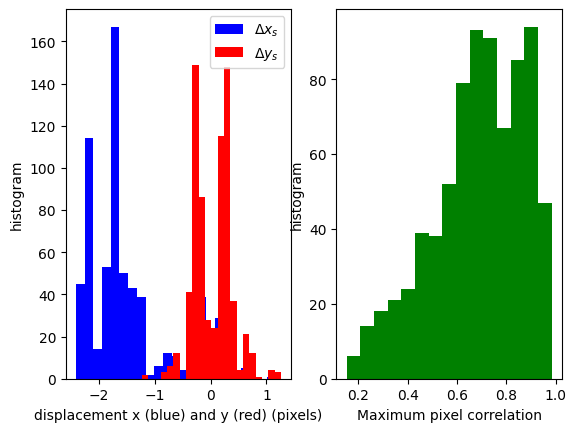
press alt+h for help and legend

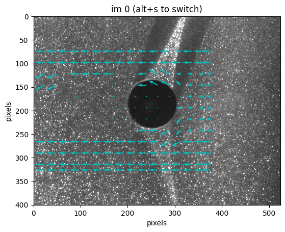
result.display(show_interp=True, show_correl=False, show_error=False);

press alt+h for help and legend

We could improve the results, but at least they seem coherent, so we can use these simple parameters with the PIV topology (usually to compute a lot of PIV fields).

Instantiate the topology and launch the computation

Let’s first import what will be useful for the computation, in particular the class fluidimage.piv.Topology.

import os

from fluidimage.piv import Topology

We use the class function create_default_params to create an object containing the parameters.

params = Topology.create_default_params()

The parameters for the PIV topology are nearly the same than those of the PIV work. One noticable difference is the addition of params.saving, because a topology saves its results. One can use _print_as_code to print parameters as in Python code (useful for copy/pasting).

params.saving._print_as_code()

saving.how = "ask"
saving.path = None
saving.postfix = "piv"

params.saving._print_doc()

Documentation for params.saving
-------------------------------

Saving of the results.

- path : None or str

  Path of the directory where the data will be saved. If None, the path is
  obtained from the input path and the parameter `postfix`.

- how : str {'ask'}

  'ask', 'new_dir', 'complete' or 'recompute'.

- postfix : str

  Postfix from which the output file is computed.

path_src = get_path_image_samples() / "Karman/Images"
params.series.path = str(path_src)

params.mask.strcrop = "50:350, 0:400"

params.piv0.shape_crop_im0 = 48
params.piv0.displacement_max = 5
params.piv0.nb_peaks_to_search = 2

params.fix.correl_min = 0.4
params.fix.threshold_diff_neighbour = 2.0

params.multipass.number = 2
params.multipass.use_tps = "last"

params.saving.how = 'recompute'
params.saving.postfix = "doc_piv_ipynb"

In order to run the PIV computation, we have to instantiate an object of the class fluidimage.piv.Topology.

topology = Topology(params)

We will then launch the computation by running the function topology.compute. For this tutorial, we use a sequential executor to get a simpler logging.

However, other Fluidimage topologies usually launch computations in parallel so that it is mandatory to set the environment variable OMP_NUM_THREADS to "1".

os.environ["OMP_NUM_THREADS"] = "1"

Let’s go!

topology.compute(sequential=True)

2024-05-02_10-26-18.27: starting execution. mem usage: 236.625 Mb
  topology: fluidimage.topologies.piv.TopologyPIV
  executor: fluidimage.executors.exec_sequential.ExecutorSequential
  nb_cpus_allowed = 2
  nb_max_workers = 4
  num_expected_results 3
  path_dir_result = /home/docs/.local/share/fluidimage/repository/image_samples/Karman/Images.doc_piv_ipynb
Monitoring app can be launched with:
fluidimage-monitor /home/docs/.local/share/fluidimage/repository/image_samples/Karman/Images.doc_piv_ipynb
Running "one_shot" job "fill (couples of names, paths)" (fluidimage.topologies.piv.fill_couples_of_names_and_paths)
INFO: Add 3 image series to compute.
INFO: Files of serie 0: ('Karman_01.bmp', 'Karman_02.bmp')
INFO: Files of serie 1: ('Karman_02.bmp', 'Karman_03.bmp')
TPS interpolation (Karman_01.bmp-Karman_02.bmp, smoothing_coef=2.0, threshold=1.5).
TPS summary: no erratic vector found.
  Statistics on the 4 TPS subdomains:
    nb_fixed_vectors  : min=0; max=0; mean=0.000
    max(Udiff)        : min=0.116; max=0.224; mean=0.157
    nb_iterations     : min=1; max=1; mean=1.000
TPS interpolation (Karman_02.bmp-Karman_03.bmp, smoothing_coef=2.0, threshold=1.5).
TPS summary: no erratic vector found.
  Statistics on the 4 TPS subdomains:
    nb_fixed_vectors  : min=0; max=0; mean=0.000
    max(Udiff)        : min=0.108; max=0.528; mean=0.220
    nb_iterations     : min=1; max=1; mean=1.000
TPS interpolation (Karman_03.bmp-Karman_04.bmp, smoothing_coef=2.0, threshold=1.5).
TPS summary: no erratic vector found.
  Statistics on the 4 TPS subdomains:
    nb_fixed_vectors  : min=0; max=0; mean=0.000
    max(Udiff)        : min=0.118; max=0.159; mean=0.136
    nb_iterations     : min=1; max=1; mean=1.000
2024-05-02_10-26-26.92: end of `compute`. mem usage: 255.426 Mb
Stop compute after t = 8.65 s (3 piv fields, 2.88 s/field, 5.76 s.CPU/field).
path results:
/home/docs/.local/share/fluidimage/repository/image_samples/Karman/Images.doc_piv_ipynb

path_src

PosixPath('/home/docs/.local/share/fluidimage/repository/image_samples/Karman/Images')

topology.path_dir_result

PosixPath('/home/docs/.local/share/fluidimage/repository/image_samples/Karman/Images.doc_piv_ipynb')

sorted(path.name for path in topology.path_dir_result.glob("*"))

['job_2024-05-02_10-26-18_1279',
 'log_2024-05-02_10-26-18_1279.txt',
 'piv_01-02.h5',
 'piv_02-03.h5',
 'piv_03-04.h5']

Fluidimage provides the command fluidpivviewer, which starts a very simple GUI to visualize the PIV results.

Analyzing the computation

from fluidimage.topologies.log import LogTopology
log = LogTopology(topology.path_dir_result)

Parsing log file: /home/docs/.local/share/fluidimage/repository/image_samples/Karman/Images.doc_piv_ipynb/log_2024-05-02_10-26-18_1279.txt
done                    

log.durations

{'read_array': [0.0, 0.0, 0.0, 0.0],
 'compute_piv': [2.871, 2.858, 2.865],
 'save_piv': [0.009, 0.01, 0.008]}

log.plot_durations()

log.plot_memory()

log.plot_nb_workers()

Loading the output files

os.chdir(topology.path_dir_result)

from fluidimage import create_object_from_file

o = create_object_from_file('piv_01-02.h5')

[s for s in dir(o) if not s.startswith('_')]

['append',
 'couple',
 'display',
 'file_name',
 'get_grid_pixel',
 'make_light_result',
 'params',
 'passes',
 'piv0',
 'piv1',
 'save']

[s for s in dir(o.piv1) if not s.startswith('_')]

['correls_max',
 'couple',
 'deltaxs',
 'deltaxs_final',
 'deltaxs_smooth',
 'deltaxs_tps',
 'deltaxs_wrong',
 'deltays',
 'deltays_final',
 'deltays_smooth',
 'deltays_tps',
 'deltays_wrong',
 'display',
 'errors',
 'get_grid_pixel',
 'get_images',
 'ixvecs_final',
 'iyvecs_final',
 'params',
 'save',
 'xs',
 'xs_smooth',
 'ys',
 'ys_smooth']

o.display();

press alt+h for help and legend

o.piv0.display(
    show_interp=False, scale=0.1, show_error=False, pourcent_histo=99, hist=False
);

press alt+h for help and legend

The output PIV files are just hdf5 files. If you just want to load the final velocity field, do it manually with h5py.

import h5py
with h5py.File("piv_01-02.h5", "r") as file:
    deltaxs_final = file["piv1/deltaxs_final"][:]

from fluidimage.postproc.vector_field import VectorFieldOnGrid

field = VectorFieldOnGrid.from_file("piv_01-02.h5")

field.display(scale=0.1);

field.gaussian_filter(sigma=1).display(scale=0.1);

from shutil import rmtree
rmtree(topology.path_dir_result, ignore_errors=True)