Tomographic reconstruction using OpenCV

Tomographic reconstruction here is performed using the class TomoMLOSCV from the module fluidimage.reconstruct.tomo.

As input we have a pair of preprocessed particle images from each of the 4 cameras. Let us start by loading the calibration data generated in the previous tutorial, and instantiating the MLOS class.

Instantiation

from fluidimage import get_path_image_samples

path = get_path_image_samples() / "TomoPIV" / "calibration"
cameras = [str(path / f"cam{i}.h5") for i in range(4)]
cameras

['/home/docs/.local/share/fluidimage/repository/image_samples/TomoPIV/calibration/cam0.h5',
 '/home/docs/.local/share/fluidimage/repository/image_samples/TomoPIV/calibration/cam1.h5',
 '/home/docs/.local/share/fluidimage/repository/image_samples/TomoPIV/calibration/cam2.h5',
 '/home/docs/.local/share/fluidimage/repository/image_samples/TomoPIV/calibration/cam3.h5']

To instantiate, we need to pass the paths of the calibration files as a list, specify limits of the world coordinates and number of voxels along each axes (i.e. the shape of the 3D volume to reconstruct).

from fluidimage.reconstruct.tomo import TomoMLOSCV


tomo = TomoMLOSCV(
        *cameras,
        xlims=(-10, 10), ylims=(-10, 10), zlims=(-5, 5), 
        nb_voxels=(20, 20, 10),
)

Install ipyvolume to visualize ArrayTomo in 3D in a Jupyter widget.
Loading /home/docs/.local/share/fluidimage/repository/image_samples/TomoPIV/calibration/cam0.h5.
Loading /home/docs/.local/share/fluidimage/repository/image_samples/TomoPIV/calibration/cam1.h5.
Loading /home/docs/.local/share/fluidimage/repository/image_samples/TomoPIV/calibration/cam2.h5.
Loading /home/docs/.local/share/fluidimage/repository/image_samples/TomoPIV/calibration/cam3.h5.

Verify projection

%matplotlib inline
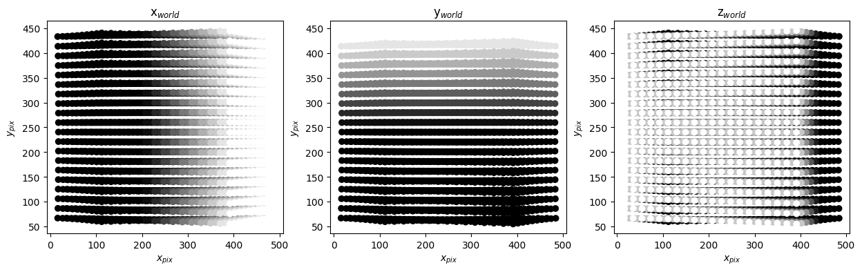
tomo.verify_projection("cam0")

tomo.verify_projection("cam3")

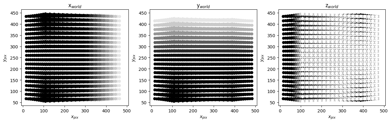
These are two cameras placed symmetrically to the left and right of \(z_{world}\) axis. As a result the projection have a left-right symmetry. So qualitatively the calibrations look correct.

Reconstruction

Setup particle_images as input and also the output directory (optional, by default a directory named tomo alongside the camera directories is set as output directory).

from pathlib import Path
from tempfile import gettempdir
import shutil

particle_images = get_path_image_samples() / "TomoPIV" / "particle"
output_dir = Path(gettempdir()) / "fluidimage_opencv_tomo_reconstruct"
if output_dir.exists():
    shutil.rmtree(output_dir)

And…. reconstruct the volume!

Note: In the next section, we reconstruct inside with the array in the memory. This is useful to visualize it immediately after the result is obtained. For larger volumes this may not be feasible, and a better option would be to reconstruct into the filesystem. Set save=True in tomo.reconstruct function to achieve that.

for cam in tomo.cams:
    print(f"Projecting {cam}...")
    pix = tomo.phys2pix(cam)
    i0 = 1
    for i1 in ["a", "b"]:
        image = str(particle_images / f"{cam}.pre" / f"im{i0:05.0f}{i1}.tif")
        tomo.array.init_paths(image, output_dir)
        print(f"MLOS of {cam} on {image}: reconstructing...")
        tomo.reconstruct(
            pix, image, threshold=None, save=False)

Projecting cam0...
MLOS of cam0 on /home/docs/.local/share/fluidimage/repository/image_samples/TomoPIV/particle/cam0.pre/im00001a.tif: reconstructing...
[########################################] | 100% Completed | 101.15 ms
MLOS of cam0 on /home/docs/.local/share/fluidimage/repository/image_samples/TomoPIV/particle/cam0.pre/im00001b.tif: reconstructing...
[########################################] | 100% Completed | 100.98 ms
Projecting cam1...
MLOS of cam1 on /home/docs/.local/share/fluidimage/repository/image_samples/TomoPIV/particle/cam1.pre/im00001a.tif: reconstructing...
[########################################] | 100% Completed | 101.49 ms
MLOS of cam1 on /home/docs/.local/share/fluidimage/repository/image_samples/TomoPIV/particle/cam1.pre/im00001b.tif: reconstructing...
[########################################] | 100% Completed | 101.05 ms
Projecting cam2...
MLOS of cam2 on /home/docs/.local/share/fluidimage/repository/image_samples/TomoPIV/particle/cam2.pre/im00001a.tif: reconstructing...
[########################################] | 100% Completed | 101.28 ms
MLOS of cam2 on /home/docs/.local/share/fluidimage/repository/image_samples/TomoPIV/particle/cam2.pre/im00001b.tif: reconstructing...
[########################################] | 100% Completed | 101.44 ms
Projecting cam3...
MLOS of cam3 on /home/docs/.local/share/fluidimage/repository/image_samples/TomoPIV/particle/cam3.pre/im00001a.tif: reconstructing...
[########################################] | 100% Completed | 101.47 ms
MLOS of cam3 on /home/docs/.local/share/fluidimage/repository/image_samples/TomoPIV/particle/cam3.pre/im00001b.tif: reconstructing...
[########################################] | 100% Completed | 100.95 ms

Visualize interactively

Plot the whole volume using a ipyvolume widget.

# import ipyvolume.pylab as p3
# fig, scatter = tomo.array.plot3d()
# p3.show()
help(tomo.array.plot3d)

Help on method plot3d in module fluidimage.data_objects.tomo:

plot3d(threshold=0.5) method of fluidimage.data_objects.tomo.ArrayTomoCV instance
    Display the reconstructed intensities as an Jupyter widget using
    ipyvolume.

Or, visualize slices along \(z_{world}\) one by one.

# %matplotlib
# tomo.array.plot_slices()
help(tomo.array.plot_slices)

Help on method plot_slices in module fluidimage.data_objects.tomo:

plot_slices(start=0, stop=None) method of fluidimage.data_objects.tomo.ArrayTomoCV instance

Footnote: The MLOS algorithm

This is how MLOS works:

1. All the points in the volume (voxels) are initialized as unity.

2. The rotation and translation vectors are linearly interpolated in z such that a particular slice where z is constant can be projected

3. All the voxels in the z-slice are projected into pixel coordinates, using the OpenCV function cv2.projectPoints which uses the expression shown in Fig. 5 which includes radial and tangential distortion compensation.

4. The projected voxels are initialized using nearest neighbour interpolation

5. The initialized voxels are re-projected back into the volume and multiplied with the previous value of the z-slice.

6. Repeat the steps for every z-slice and for every camera.

7. Normalize the final intensities by raising them to the power of \(1/N_{cam}\).

The relevant function which performs the projection is TomoMLOSCV.phys2pix and TomoMLOSCV.get_interpolator and TomoMLOSCV.reconstruct does calculates the interpolation and applies MLOS back-projection, respectively.